Apart from training/testing scripts, We provide lots of useful tools under the
tools/ directory.
Log Analysis
tools/analysis_tools/analyze_logs.py plots loss/mAP curves given a training
log file. Run pip install seaborn first to install the dependency.
python tools/analysis_tools/analyze_logs.py plot_curve [--keys ${KEYS}] [--title ${TITLE}] [--legend ${LEGEND}] [--backend ${BACKEND}] [--style ${STYLE}] [--out ${OUT_FILE}]
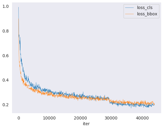 loss curve image
Examples:
Plot the classification loss of some run.
python tools/analysis_tools/analyze_logs.py plot_curve log.json --keys loss_cls --legend loss_cls
Plot the classification and regression loss of some run, and save the figure to a pdf.
python tools/analysis_tools/analyze_logs.py plot_curve log.json --keys loss_cls loss_bbox --out losses.pdf
Compare the bbox mAP of two runs in the same figure.
python tools/analysis_tools/analyze_logs.py plot_curve log1.json log2.json --keys bbox_mAP --legend run1 run2
Compute the average training speed.
python tools/analysis_tools/analyze_logs.py cal_train_time log.json [--include-outliers]
The output is expected to be like the following.
-----Analyze train time of work_dirs/some_exp/20190611_192040.log.json-----
slowest epoch 11, average time is 1.2024
fastest epoch 1, average time is 1.1909
time std over epochs is 0.0028
average iter time: 1.1959 s/iter
Result Analysis
tools/analysis_tools/analyze_results.py calculates single image mAP and saves or shows the topk images with the highest and lowest scores based on prediction results.
Usage
python tools/analysis_tools/analyze_results.py \
      ${CONFIG} \
      ${PREDICTION_PATH} \
      ${SHOW_DIR} \
      [--show] \
      [--wait-time ${WAIT_TIME}] \
      [--topk ${TOPK}] \
      [--show-score-thr ${SHOW_SCORE_THR}] \
      [--cfg-options ${CFG_OPTIONS}]
Description of all arguments:
config: The path of a model config file.prediction_path: Output result file in pickle format fromtools/test.pyshow_dir: Directory where painted GT and detection images will be saved--show:Determines whether to show painted images, If not specified, it will be set toFalse--wait-time: The interval of show (s), 0 is block--topk: The number of saved images that have the highest and lowesttopkscores after sorting. If not specified, it will be set to20.--show-score-thr: Show score threshold. If not specified, it will be set to0.--cfg-options: If specified, the key-value pair optional cfg will be merged into config file
Examples:
Assume that you have got result file in pickle format from tools/test.py in the path ‘./result.pkl’.
- Test Faster R-CNN and visualize the results, save images to the directory
results/
python tools/analysis_tools/analyze_results.py \
       configs/faster_rcnn/faster_rcnn_r50_fpn_1x_coco.py \
       result.pkl \
       results \
       --show
- Test Faster R-CNN and specified topk to 50, save images to the directory
results/
python tools/analysis_tools/analyze_results.py \
       configs/faster_rcnn/faster_rcnn_r50_fpn_1x_coco.py \
       result.pkl \
       results \
       --topk 50
- If you want to filter the low score prediction results, you can specify the
show-score-thrparameter
python tools/analysis_tools/analyze_results.py \
       configs/faster_rcnn/faster_rcnn_r50_fpn_1x_coco.py \
       result.pkl \
       results \
       --show-score-thr 0.3
Visualization
Visualize Datasets
tools/misc/browse_dataset.py helps the user to browse a detection dataset (both
images and bounding box annotations) visually, or save the image to a
designated directory.
python tools/misc/browse_dataset.py ${CONFIG} [-h] [--skip-type ${SKIP_TYPE[SKIP_TYPE...]}] [--output-dir ${OUTPUT_DIR}] [--not-show] [--show-interval ${SHOW_INTERVAL}]
Visualize Models
First, convert the model to ONNX as described here. Note that currently only RetinaNet is supported, support for other models will be coming in later versions. The converted model could be visualized by tools like Netron.
Visualize Predictions
If you need a lightweight GUI for visualizing the detection results, you can refer DetVisGUI project.
Error Analysis
tools/analysis_tools/coco_error_analysis.py analyzes COCO results per category and by
different criterion. It can also make a plot to provide useful information.
python tools/analysis_tools/coco_error_analysis.py ${RESULT} ${OUT_DIR} [-h] [--ann ${ANN}] [--types ${TYPES[TYPES...]}]
Example:
Assume that you have got Mask R-CNN checkpoint file in the path ‘checkpoint’. For other checkpoints, please refer to our model zoo. You can use the following command to get the results bbox and segmentation json file.
# out: results.bbox.json and results.segm.json
python tools/test.py \
       configs/mask_rcnn/mask_rcnn_r50_fpn_1x_coco.py \
       checkpoint/mask_rcnn_r50_fpn_1x_coco_20200205-d4b0c5d6.pth \
       --format-only \
       --options "jsonfile_prefix=./results"
- Get COCO bbox error results per category , save analyze result images to the directory
results/
python tools/analysis_tools/coco_error_analysis.py \
       results.bbox.json \
       results \
       --ann=data/coco/annotations/instances_val2017.json \
- Get COCO segmentation error results per category , save analyze result images to the directory
results/
python tools/analysis_tools/coco_error_analysis.py \
       results.segm.json \
       results \
       --ann=data/coco/annotations/instances_val2017.json \
       --types='segm'
Model Serving
In order to serve an MMDetection model with TorchServe, you can follow the steps:
1. Convert model from MMDetection to TorchServe
python tools/deployment/mmdet2torchserve.py ${CONFIG_FILE} ${CHECKPOINT_FILE} \
--output-folder ${MODEL_STORE} \
--model-name ${MODEL_NAME}
Note: ${MODEL_STORE} needs to be an absolute path to a folder.
2. Build mmdet-serve docker image
docker build -t mmdet-serve:latest docker/serve/
3. Run mmdet-serve
Check the official docs for running TorchServe with docker.
In order to run in GPU, you need to install nvidia-docker. You can omit the --gpus argument in order to run in CPU.
Example:
docker run --rm \
--cpus 8 \
--gpus device=0 \
-p8080:8080 -p8081:8081 -p8082:8082 \
--mount type=bind,source=$MODEL_STORE,target=/home/model-server/model-store \
mmdet-serve:latest
Read the docs about the Inference (8080), Management (8081) and Metrics (8082) APis
4. Test deployment
curl -O curl -O https://raw.githubusercontent.com/pytorch/serve/master/docs/images/3dogs.jpg
curl http://127.0.0.1:8080/predictions/${MODEL_NAME} -T 3dogs.jpg
You should obtain a respose similar to:
[
  {
    "dog": [
      402.9117736816406,
      124.19664001464844,
      571.7910766601562,
      292.6463623046875
    ],
    "score": 0.9561963081359863
  },
  {
    "dog": [
      293.90057373046875,
      196.2908477783203,
      417.4869079589844,
      286.2522277832031
    ],
    "score": 0.9179860353469849
  },
  {
    "dog": [
      202.178466796875,
      86.3709487915039,
      311.9863586425781,
      276.28411865234375
    ],
    "score": 0.8933767080307007
  }
]
Model Complexity
tools/analysis_tools/get_flops.py is a script adapted from flops-counter.pytorch to compute the FLOPs and params of a given model.
python tools/analysis_tools/get_flops.py ${CONFIG_FILE} [--shape ${INPUT_SHAPE}]
You will get the results like this.
==============================
Input shape: (3, 1280, 800)
Flops: 239.32 GFLOPs
Params: 37.74 M
==============================
Note: This tool is still experimental and we do not guarantee that the number is absolutely correct. You may well use the result for simple comparisons, but double check it before you adopt it in technical reports or papers.
- FLOPs are related to the input shape while parameters are not. The default input shape is (1, 3, 1280, 800).
- Some operators are not counted into FLOPs like GN and custom operators. Refer to
mmcv.cnn.get_model_complexity_info()for details. - The FLOPs of two-stage detectors is dependent on the number of proposals.
Model conversion
MMDetection model to ONNX (experimental)
We provide a script to convert model to ONNX format. We also support comparing the output results between Pytorch and ONNX model for verification.
python tools/deployment/pytorch2onnx.py ${CONFIG_FILE} ${CHECKPOINT_FILE} --output_file ${ONNX_FILE} [--shape ${INPUT_SHAPE} --verify]
Note: This tool is still experimental. Some customized operators are not supported for now. For a detailed description of the usage and the list of supported models, please refer to pytorch2onnx.
MMDetection 1.x model to MMDetection 2.x
tools/model_converters/upgrade_model_version.py upgrades a previous MMDetection checkpoint
to the new version. Note that this script is not guaranteed to work as some
breaking changes are introduced in the new version. It is recommended to
directly use the new checkpoints.
python tools/model_converters/upgrade_model_version.py ${IN_FILE} ${OUT_FILE} [-h] [--num-classes NUM_CLASSES]
RegNet model to MMDetection
tools/model_converters/regnet2mmdet.py convert keys in pycls pretrained RegNet models to
MMDetection style.
python tools/model_converters/regnet2mmdet.py ${SRC} ${DST} [-h]
Detectron ResNet to Pytorch
tools/model_converters/detectron2pytorch.py converts keys in the original detectron pretrained
ResNet models to PyTorch style.
python tools/model_converters/detectron2pytorch.py ${SRC} ${DST} ${DEPTH} [-h]
Prepare a model for publishing
tools/model_converters/publish_model.py helps users to prepare their model for publishing.
Before you upload a model to AWS, you may want to
- convert model weights to CPU tensors
- delete the optimizer states and
- compute the hash of the checkpoint file and append the hash id to the filename.
python tools/model_converters/publish_model.py ${INPUT_FILENAME} ${OUTPUT_FILENAME}
E.g.,
python tools/model_converters/publish_model.py work_dirs/faster_rcnn/latest.pth faster_rcnn_r50_fpn_1x_20190801.pth
The final output filename will be faster_rcnn_r50_fpn_1x_20190801-{hash id}.pth.
Dataset Conversion
tools/data_converters/ contains tools to convert the Cityscapes dataset
and Pascal VOC dataset to the COCO format.
python tools/dataset_converters/cityscapes.py ${CITYSCAPES_PATH} [-h] [--img-dir ${IMG_DIR}] [--gt-dir ${GT_DIR}] [-o ${OUT_DIR}] [--nproc ${NPROC}]
python tools/dataset_converters/pascal_voc.py ${DEVKIT_PATH} [-h] [-o ${OUT_DIR}]
Robust Detection Benchmark
tools/analysis_tools/test_robustness.py andtools/analysis_tools/robustness_eval.py helps users to evaluate model robustness. The core idea comes from Benchmarking Robustness in Object Detection: Autonomous Driving when Winter is Coming. For more information how to evaluate models on corrupted images and results for a set of standard models please refer to robustness_benchmarking.md.
Miscellaneous
Evaluating a metric
tools/analysis_tools/eval_metric.py evaluates certain metrics of a pkl result file
according to a config file.
python tools/analysis_tools/eval_metric.py ${CONFIG} ${PKL_RESULTS} [-h] [--format-only] [--eval ${EVAL[EVAL ...]}]
                      [--cfg-options ${CFG_OPTIONS [CFG_OPTIONS ...]}]
                      [--eval-options ${EVAL_OPTIONS [EVAL_OPTIONS ...]}]
Print the entire config
tools/misc/print_config.py prints the whole config verbatim, expanding all its
imports.
python tools/misc/print_config.py ${CONFIG} [-h] [--options ${OPTIONS [OPTIONS...]}]
Hyper-parameter Optimization
YOLO Anchor Optimization
tools/analysis_tools/optimize_anchors.py provides two method to optimize YOLO anchors.
One is k-means anchor cluster which refers from darknet.
python tools/analysis_tools/optimize_anchors.py ${CONFIG} --algorithm k-means --input-shape ${INPUT_SHAPE [WIDTH HEIGHT]} --output-dir ${OUTPUT_DIR}
Another is using differential evolution to optimize anchors.
python tools/analysis_tools/optimize_anchors.py ${CONFIG} --algorithm differential_evolution --input-shape ${INPUT_SHAPE [WIDTH HEIGHT]} --output-dir ${OUTPUT_DIR}
E.g.,
python tools/analysis_tools/optimize_anchors.py configs/yolo/yolov3_d53_320_273e_coco.py --algorithm differential_evolution --input-shape 608 608 --device cuda --output-dir work_dirs
You will get:
loading annotations into memory...
Done (t=9.70s)
creating index...
index created!
2021-07-19 19:37:20,951 - mmdet - INFO - Collecting bboxes from annotation...
[>>>>>>>>>>>>>>>>>>>>>>>>>>>>>>>>>>>>>>>>>>>>>>>>>>] 117266/117266, 15874.5 task/s, elapsed: 7s, ETA:     0s

2021-07-19 19:37:28,753 - mmdet - INFO - Collected 849902 bboxes.
differential_evolution step 1: f(x)= 0.506055
differential_evolution step 2: f(x)= 0.506055
......

differential_evolution step 489: f(x)= 0.386625
2021-07-19 19:46:40,775 - mmdet - INFO Anchor evolution finish. Average IOU: 0.6133754253387451
2021-07-19 19:46:40,776 - mmdet - INFO Anchor differential evolution result:[[10, 12], [15, 30], [32, 22], [29, 59], [61, 46], [57, 116], [112, 89], [154, 198], [349, 336]]
2021-07-19 19:46:40,798 - mmdet - INFO Result saved in work_dirs/anchor_optimize_result.json