Getting Started
This page provides basic tutorials about the usage of MMDetection. For installation instructions, please see INSTALL.md.
Inference with pretrained models
We provide testing scripts to evaluate a whole dataset (COCO, PASCAL VOC, Cityscapes, etc.), and also some high-level apis for easier integration to other projects.
Test a dataset
- [x] single GPU testing
- [x] multiple GPU testing
- [x] visualize detection results
You can use the following commands to test a dataset.
# single-gpu testing
python tools/test.py ${CONFIG_FILE} ${CHECKPOINT_FILE} [--out ${RESULT_FILE}] [--eval ${EVAL_METRICS}] [--show]

# multi-gpu testing
./tools/dist_test.sh ${CONFIG_FILE} ${CHECKPOINT_FILE} ${GPU_NUM} [--out ${RESULT_FILE}] [--eval ${EVAL_METRICS}]
Optional arguments:
RESULT_FILE: Filename of the output results in pickle format. If not specified, the results will not be saved to a file.EVAL_METRICS: Items to be evaluated on the results. Allowed values depend on the dataset, e.g.,proposal_fast,proposal,bbox,segmare available for COCO,mAP,recallfor PASCAL VOC. Cityscapes could be evaluated bycityscapesas well as all COCO metrics.--show: If specified, detection results will be plotted on the images and shown in a new window. It is only applicable to single GPU testing and used for debugging and visualization. Please make sure that GUI is available in your environment, otherwise you may encounter the error likecannot connect to X server.
If you would like to evaluate the dataset, do not specify --show at the same time.
Examples:
Assume that you have already downloaded the checkpoints to the directory checkpoints/.
- Test Faster R-CNN and visualize the results. Press any key for the next image.
python tools/test.py configs/faster_rcnn_r50_fpn_1x.py \
    checkpoints/faster_rcnn_r50_fpn_1x_20181010-3d1b3351.pth \
    --show
- Test Faster R-CNN on PASCAL VOC (without saving the test results) and evaluate the mAP.
python tools/test.py configs/pascal_voc/faster_rcnn_r50_fpn_1x_voc.py \
    checkpoints/SOME_CHECKPOINT.pth \
    --eval mAP
- Test Mask R-CNN with 8 GPUs, and evaluate the bbox and mask AP.
./tools/dist_test.sh configs/mask_rcnn_r50_fpn_1x.py \
    checkpoints/mask_rcnn_r50_fpn_1x_20181010-069fa190.pth \
    8 --out results.pkl --eval bbox segm
- Test Mask R-CNN on COCO test-dev with 8 GPUs, and generate the json file to be submit to the official evaluation server.
./tools/dist_test.sh configs/mask_rcnn_r50_fpn_1x.py \
    checkpoints/mask_rcnn_r50_fpn_1x_20181010-069fa190.pth \
    8 --format_only --options "jsonfile_prefix=./mask_rcnn_test-dev_results"
You will get two json files mask_rcnn_test-dev_results.bbox.json and mask_rcnn_test-dev_results.segm.json.
- Test Mask R-CNN on Cityscapes test with 8 GPUs, and generate the txt and png files to be submit to the official evaluation server.
./tools/dist_test.sh configs/cityscapes/mask_rcnn_r50_fpn_1x_cityscapes.py \
    checkpoints/mask_rcnn_r50_fpn_1x_cityscapes_20200227-afe51d5a.pth \
    8  --format_only --options "txtfile_prefix=./mask_rcnn_cityscapes_test_results"
The generated png and txt would be under ./mask_rcnn_cityscapes_test_results directory.
Webcam demo
We provide a webcam demo to illustrate the results.
python demo/webcam_demo.py ${CONFIG_FILE} ${CHECKPOINT_FILE} [--device ${GPU_ID}] [--camera-id ${CAMERA-ID}] [--score-thr ${SCORE_THR}]
Examples:
python demo/webcam_demo.py configs/faster_rcnn_r50_fpn_1x.py \
    checkpoints/faster_rcnn_r50_fpn_1x_20181010-3d1b3351.pth
High-level APIs for testing images
Synchronous interface
Here is an example of building the model and test given images.
from mmdet.apis import init_detector, inference_detector, show_result
import mmcv

config_file = 'configs/faster_rcnn_r50_fpn_1x.py'
checkpoint_file = 'checkpoints/faster_rcnn_r50_fpn_1x_20181010-3d1b3351.pth'

# build the model from a config file and a checkpoint file
model = init_detector(config_file, checkpoint_file, device='cuda:0')

# test a single image and show the results
img = 'test.jpg'  # or img = mmcv.imread(img), which will only load it once
result = inference_detector(model, img)
# visualize the results in a new window
show_result(img, result, model.CLASSES)
# or save the visualization results to image files
show_result(img, result, model.CLASSES, out_file='result.jpg')

# test a video and show the results
video = mmcv.VideoReader('video.mp4')
for frame in video:
    result = inference_detector(model, frame)
    show_result(frame, result, model.CLASSES, wait_time=1)
A notebook demo can be found in demo/inference_demo.ipynb.
Asynchronous interface - supported for Python 3.7+
Async interface allows not to block CPU on GPU bound inference code and enables better CPU/GPU utilization for single threaded application. Inference can be done concurrently either between different input data samples or between different models of some inference pipeline.
See tests/async_benchmark.py to compare the speed of synchronous and asynchronous interfaces.
import asyncio
import torch
from mmdet.apis import init_detector, async_inference_detector, show_result
from mmdet.utils.contextmanagers import concurrent

async def main():
    config_file = 'configs/faster_rcnn_r50_fpn_1x.py'
    checkpoint_file = 'checkpoints/faster_rcnn_r50_fpn_1x_20181010-3d1b3351.pth'
    device = 'cuda:0'
    model = init_detector(config_file, checkpoint=checkpoint_file, device=device)

    # queue is used for concurrent inference of multiple images
    streamqueue = asyncio.Queue()
    # queue size defines concurrency level
    streamqueue_size = 3

    for _ in range(streamqueue_size):
        streamqueue.put_nowait(torch.cuda.Stream(device=device))

    # test a single image and show the results
    img = 'test.jpg'  # or img = mmcv.imread(img), which will only load it once

    async with concurrent(streamqueue):
        result = await async_inference_detector(model, img)

    # visualize the results in a new window
    show_result(img, result, model.CLASSES)
    # or save the visualization results to image files
    show_result(img, result, model.CLASSES, out_file='result.jpg')

asyncio.run(main())
Train a model
MMDetection implements distributed training and non-distributed training,
which uses MMDistributedDataParallel and MMDataParallel respectively.
All outputs (log files and checkpoints) will be saved to the working directory,
which is specified by work_dir in the config file.
By default we evaluate the model on the validation set after each epoch, you can change the evaluation interval by adding the interval argument in the training config.
evaluation = dict(interval=12) # This evaluate the model per 12 epoch.
*Important*: The default learning rate in config files is for 8 GPUs and 2 img/gpu (batch size = 8*2 = 16). According to the Linear Scaling Rule, you need to set the learning rate proportional to the batch size if you use different GPUs or images per GPU, e.g., lr=0.01 for 4 GPUs * 2 img/gpu and lr=0.08 for 16 GPUs * 4 img/gpu.
Train with a single GPU
python tools/train.py ${CONFIG_FILE} [optional arguments]
If you want to specify the working directory in the command, you can add an argument --work_dir ${YOUR_WORK_DIR}.
Train with multiple GPUs
./tools/dist_train.sh ${CONFIG_FILE} ${GPU_NUM} [optional arguments]
Optional arguments are:
--validate(strongly recommended): Perform evaluation at every k (default value is 1, which can be modified like this) epochs during the training.--work_dir ${WORK_DIR}: Override the working directory specified in the config file.--resume_from ${CHECKPOINT_FILE}: Resume from a previous checkpoint file.
Difference between resume_from and load_from:
resume_from loads both the model weights and optimizer status, and the epoch is also inherited from the specified checkpoint. It is usually used for resuming the training process that is interrupted accidentally.
load_from only loads the model weights and the training epoch starts from 0. It is usually used for finetuning.
Train with multiple machines
If you run MMDetection on a cluster managed with slurm, you can use the script slurm_train.sh. (This script also supports single machine training.)
./tools/slurm_train.sh ${PARTITION} ${JOB_NAME} ${CONFIG_FILE} ${WORK_DIR} [${GPUS}]
Here is an example of using 16 GPUs to train Mask R-CNN on the dev partition.
./tools/slurm_train.sh dev mask_r50_1x configs/mask_rcnn_r50_fpn_1x.py /nfs/xxxx/mask_rcnn_r50_fpn_1x 16
You can check slurm_train.sh for full arguments and environment variables.
If you have just multiple machines connected with ethernet, you can refer to pytorch launch utility. Usually it is slow if you do not have high speed networking like infiniband.
Launch multiple jobs on a single machine
If you launch multiple jobs on a single machine, e.g., 2 jobs of 4-GPU training on a machine with 8 GPUs, you need to specify different ports (29500 by default) for each job to avoid communication conflict.
If you use dist_train.sh to launch training jobs, you can set the port in commands.
CUDA_VISIBLE_DEVICES=0,1,2,3 PORT=29500 ./tools/dist_train.sh ${CONFIG_FILE} 4
CUDA_VISIBLE_DEVICES=4,5,6,7 PORT=29501 ./tools/dist_train.sh ${CONFIG_FILE} 4
If you use launch training jobs with slurm, you need to modify the config files (usually the 6th line from the bottom in config files) to set different communication ports.
In config1.py,
dist_params = dict(backend='nccl', port=29500)
In config2.py,
dist_params = dict(backend='nccl', port=29501)
Then you can launch two jobs with config1.py ang config2.py.
CUDA_VISIBLE_DEVICES=0,1,2,3 ./tools/slurm_train.sh ${PARTITION} ${JOB_NAME} config1.py ${WORK_DIR} 4
CUDA_VISIBLE_DEVICES=4,5,6,7 ./tools/slurm_train.sh ${PARTITION} ${JOB_NAME} config2.py ${WORK_DIR} 4
Useful tools
We provide lots of useful tools under tools/ directory.
Analyze logs
You can plot loss/mAP curves given a training log file. Run pip install seaborn first to install the dependency.
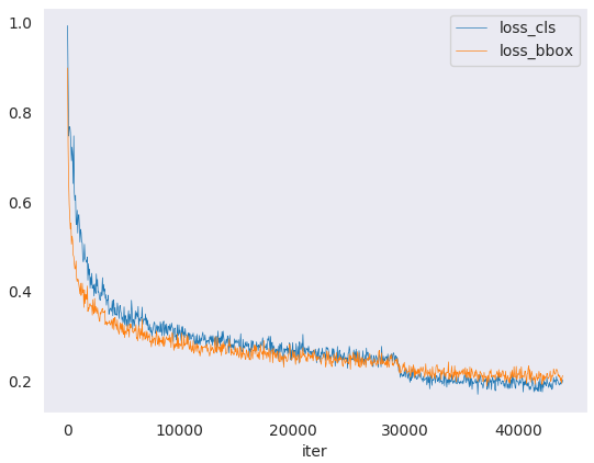 loss curve image
python tools/analyze_logs.py plot_curve [--keys ${KEYS}] [--title ${TITLE}] [--legend ${LEGEND}] [--backend ${BACKEND}] [--style ${STYLE}] [--out ${OUT_FILE}]
Examples:
- Plot the classification loss of some run.
python tools/analyze_logs.py plot_curve log.json --keys loss_cls --legend loss_cls
- Plot the classification and regression loss of some run, and save the figure to a pdf.
python tools/analyze_logs.py plot_curve log.json --keys loss_cls loss_reg --out losses.pdf
- Compare the bbox mAP of two runs in the same figure.
python tools/analyze_logs.py plot_curve log1.json log2.json --keys bbox_mAP --legend run1 run2
You can also compute the average training speed.
python tools/analyze_logs.py cal_train_time ${CONFIG_FILE} [--include-outliers]
The output is expected to be like the following.
-----Analyze train time of work_dirs/some_exp/20190611_192040.log.json-----
slowest epoch 11, average time is 1.2024
fastest epoch 1, average time is 1.1909
time std over epochs is 0.0028
average iter time: 1.1959 s/iter
Get the FLOPs and params (experimental)
We provide a script adapted from flops-counter.pytorch to compute the FLOPs and params of a given model.
python tools/get_flops.py ${CONFIG_FILE} [--shape ${INPUT_SHAPE}]
You will get the result like this.
==============================
Input shape: (3, 1280, 800)
Flops: 239.32 GMac
Params: 37.74 M
==============================
Note: This tool is still experimental and we do not guarantee that the number is correct. You may well use the result for simple comparisons, but double check it before you adopt it in technical reports or papers.
(1) FLOPs are related to the input shape while parameters are not. The default input shape is (1, 3, 1280, 800).
(2) Some operators are not counted into FLOPs like GN and custom operators.
You can add support for new operators by modifying mmdet/utils/flops_counter.py.
(3) The FLOPs of two-stage detectors is dependent on the number of proposals.
Publish a model
Before you upload a model to AWS, you may want to (1) convert model weights to CPU tensors, (2) delete the optimizer states and (3) compute the hash of the checkpoint file and append the hash id to the filename.
python tools/publish_model.py ${INPUT_FILENAME} ${OUTPUT_FILENAME}
E.g.,
python tools/publish_model.py work_dirs/faster_rcnn/latest.pth faster_rcnn_r50_fpn_1x_20190801.pth
The final output filename will be faster_rcnn_r50_fpn_1x_20190801-{hash id}.pth.
Test the robustness of detectors
Please refer to ROBUSTNESS_BENCHMARKING.md.
Convert to ONNX (experimental)
We provide a script to convert model to ONNX format. The converted model could be visualized by tools like Netron.
python tools/pytorch2onnx.py ${CONFIG_FILE} ${CHECKPOINT_FILE} --out ${ONNX_FILE} [--shape ${INPUT_SHAPE}]
Note: This tool is still experimental. Customized operators are not supported for now. We set use_torchvision=True on-the-fly for RoIPool and RoIAlign.
How-to
Use my own datasets
The simplest way is to convert your dataset to existing dataset formats (COCO or PASCAL VOC).
Here we show an example of adding a custom dataset of 5 classes, assuming it is also in COCO format.
In mmdet/datasets/my_dataset.py:
from .coco import CocoDataset
from .registry import DATASETS

@DATASETS.register_module
class MyDataset(CocoDataset):

    CLASSES = ('a', 'b', 'c', 'd', 'e')
In mmdet/datasets/__init__.py:
from .my_dataset import MyDataset
Then you can use MyDataset in config files, with the same API as CocoDataset.
It is also fine if you do not want to convert the annotation format to COCO or PASCAL format. Actually, we define a simple annotation format and all existing datasets are processed to be compatible with it, either online or offline.
The annotation of a dataset is a list of dict, each dict corresponds to an image.
There are 3 field filename (relative path), width, height for testing,
and an additional field ann for training. ann is also a dict containing at least 2 fields:
bboxes and labels, both of which are numpy arrays. Some datasets may provide
annotations like crowd/difficult/ignored bboxes, we use bboxes_ignore and labels_ignore
to cover them.
Here is an example.
[
    {
        'filename': 'a.jpg',
        'width': 1280,
        'height': 720,
        'ann': {
            'bboxes': <np.ndarray, float32> (n, 4),
            'labels': <np.ndarray, int64> (n, ),
            'bboxes_ignore': <np.ndarray, float32> (k, 4),
            'labels_ignore': <np.ndarray, int64> (k, ) (optional field)
        }
    },
    ...
]
There are two ways to work with custom datasets.
online conversion
You can write a new Dataset class inherited from
CustomDataset, and overwrite two methodsload_annotations(self, ann_file)andget_ann_info(self, idx), like CocoDataset and VOCDataset.offline conversion
You can convert the annotation format to the expected format above and save it to a pickle or json file, like pascal_voc.py. Then you can simply use
CustomDataset.
Customize optimizer
An example of customized optimizer CopyOfSGD is defined in mmdet/core/optimizer/copy_of_sgd.py.
More generally, a customized optimizer could be defined as following.
In mmdet/core/optimizer/my_optimizer.py:
from .registry import OPTIMIZERS
from torch.optim import Optimizer

@OPTIMIZERS.register_module
class MyOptimizer(Optimizer):
In mmdet/core/optimizer/__init__.py:
from .my_optimizer import MyOptimizer
Then you can use MyOptimizer in optimizer field of config files.
Develop new components
We basically categorize model components into 4 types.
- backbone: usually an FCN network to extract feature maps, e.g., ResNet, MobileNet.
- neck: the component between backbones and heads, e.g., FPN, PAFPN.
- head: the component for specific tasks, e.g., bbox prediction and mask prediction.
- roi extractor: the part for extracting RoI features from feature maps, e.g., RoI Align.
Here we show how to develop new components with an example of MobileNet.
- Create a new file
mmdet/models/backbones/mobilenet.py.
import torch.nn as nn

from ..registry import BACKBONES

@BACKBONES.register_module
class MobileNet(nn.Module):

    def __init__(self, arg1, arg2):
        pass

    def forward(self, x):  # should return a tuple
        pass

    def init_weights(self, pretrained=None):
        pass
- Import the module in
mmdet/models/backbones/__init__.py.
from .mobilenet import MobileNet
- Use it in your config file.
model = dict(
    ...
    backbone=dict(
        type='MobileNet',
        arg1=xxx,
        arg2=xxx),
    ...
For more information on how it works, you can refer to TECHNICAL_DETAILS.md (TODO).